State Space Analysis for SEPIC
State Space analysis is a method used for representing nonlinear systems as a sum of linear equations [4]. This type of analysis provides a mathematical model of the system as a system of linear equations in which the transfer function of the SEPIC can be obtained. The State Space Averaging (SSA) method will be used to obtain the final representation of the SEPIC as will be explained in the next few pages. The transfer function will first be obtained to obtain a constant voltage. Once the results are obtained and a controller was designed successfully, the analysis would be extended to design a controller to obtain a constant current at the output of the SEPIC converter.
State Space Matrices for Output Voltage:
The first state-space analysis will be used to obtain the transfer function of the SEPIC where the input parameter is the supplied voltage, and the output parameter is the output voltage. The following equations are representing the standard form of state-space analysis.

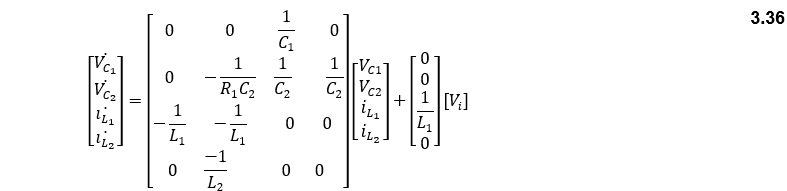
Where both equations (3.22) are the state of the system while the equation (3.23) is the output of the system. Since switching has two states (ON-OFF), the state space analysis has been done for two different states. Note that, the mutual inductances (M12, M21) are neglected because the model has winded without any dot convention. When the switch is closed, the state space equations will be:
Then, the state space matrix will be:
The output equation of the system when the switch is closed:

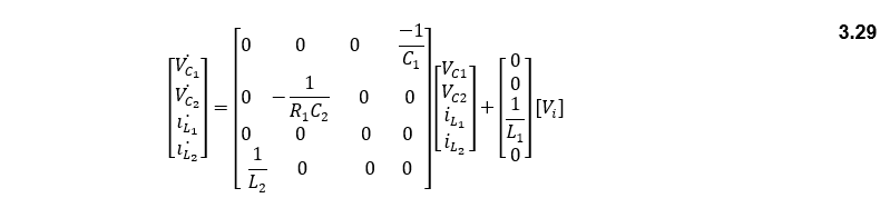
On the other hand, when the switch is open, the state space equations will be:
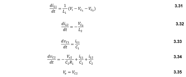
Then, the state space matrix will be:
The output equation of the system when the switch is opened:

After finding the state-space modelling for the two cases (closed and open) switches, the averaging method of state-space with variable duty cycle will be:
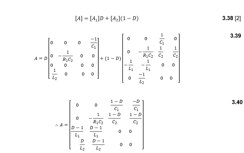
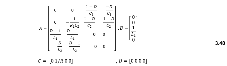
And the matrix B will be:

Where matrix C and D are for both cases:
![]()
Now, according to the use of the SSA in the block diagram representing the closed-loop SEPIC shown below. The transfer function that is needed to be obtained is the duty cycle to output voltage transfer function (Vo/d) since the input to the plant is the averaged duty cycle from the controller.
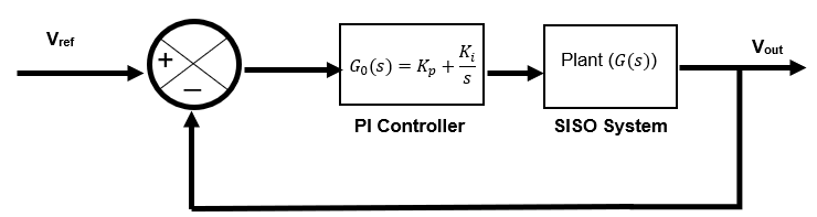
Figure 3‑20: The closed Loop System.
Equations (3.22) and (3.23) are nonlinear; that is why a small signal perturbation is used to linearize the signals where x, y, vi, and d (duty cycle) are represented by a capital letter for constant values and the symbol ~ for representing the small changing signal [53]. According to [53], the control to output voltage transfer function is:

Where :
![]()
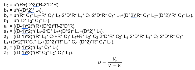
Note that the duty cycle that is included in the A matrix, and the X matrix are both constant (DC) values. Thus, the duty cycle is calculated directly through the input voltage/output voltage relation, while the varying duty cycle is the one that inters the plant using the controller. The resulting transfer function is:

Where :
Now, the values of the components are as selected earlier:

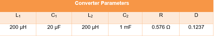
Now, Vo= 48 V, Vi= 340 V, Po= 4 kW, dVc1= 0.05(Vi), dVo/Vo= 0.01. So, all the inductors and capacitors values chosen for the SEPIC from the comparison between (Boost, Cuk, and SEPIC), meet the specifications made above except for C1. The new values are shown in the table below.
Table 3‑7 SEPIC converter parameters when at constant voltage method.

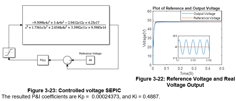
Now, this transfer function is modelled in the MATLAB and both the poles and zeros of the transfer function were plotted using the root locus method. Later, a compensator was added that should represent the varying duty cycle to get the desired output. Then by changing the small acting poles and zeros, the best step response was obtained, and the resulting P&I coefficients are used to simulate the mathematical model in Simulink.
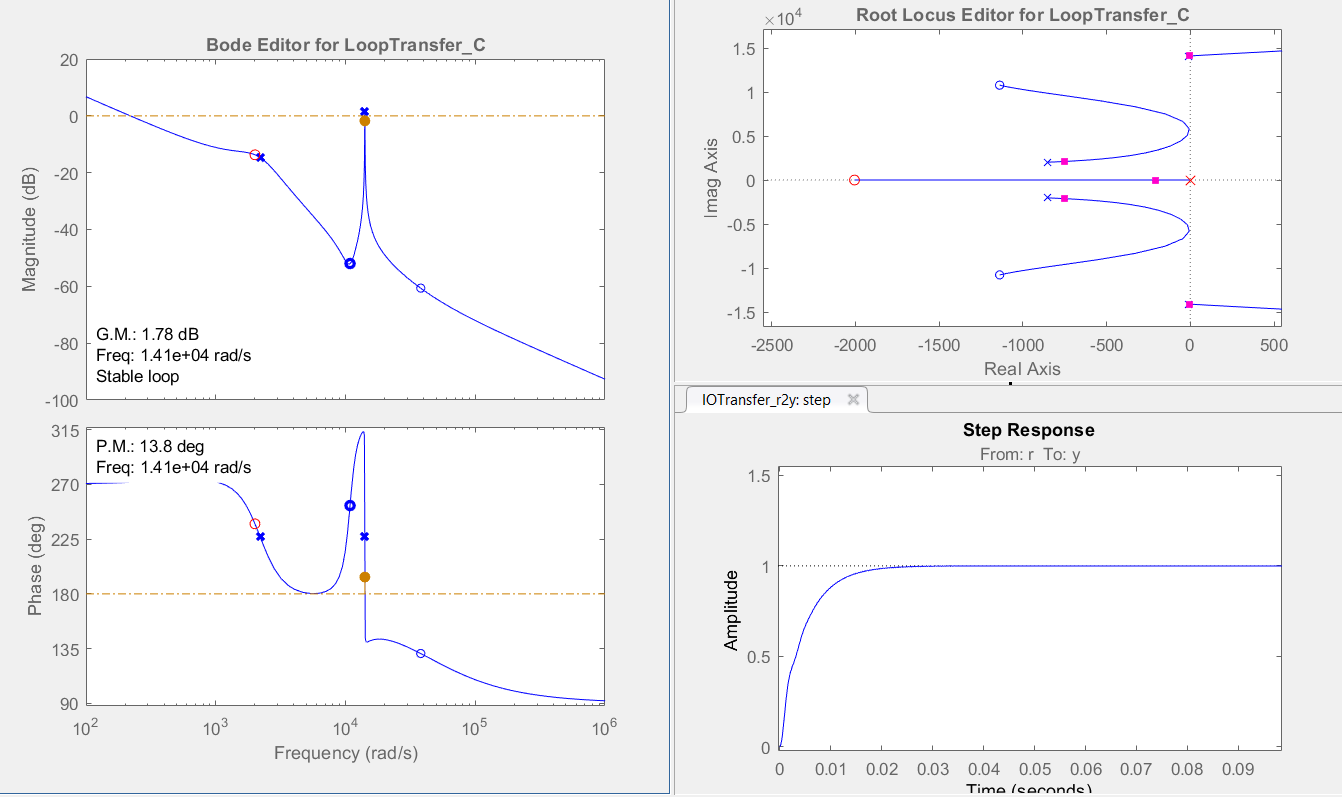
Figure 3‑21: Root locus for Controlled Voltage SEPIC.
State Space Matrices for Output Current:
Now, state-space matrices are going to be developed for the SEPIC converter when the output is the load current. This is important for the development of a controlled current SEPIC converter since that would lead to a constant power charging for the battery since the battery’s voltage is already constant. The approach for deriving the state space for the output current is the same as for the output voltage, since all the system variables, and system input are the same. Therefore, the equation for the state of the system is the same as equations (3.29) and (3.36). thus, the averaged A and B are equal to Equations (3.40) and (3.42) consecutively. The equation for the output of the system is the same for both the switching on/off conditions which is:

So, the value of the averaged A, B, C, and D are:
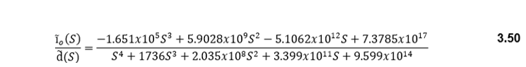
The equation to obtain the duty cycle to output the current transfer function is the same as the duty cycle to output voltage transfer function. Therefore (Io/d) is:

where :

All the passive element’s values are the same as in table 3.5. the transfer function is:
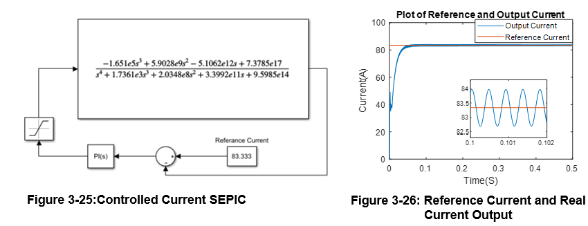
Now, the goal is to obtain a stable system and yet reach steady-state very swiftly. A PI compensator will be added before the plant, to obtain the optimum results as shown in figure (1). Now, the root locus method will be used to obtain the poles and zeros of the open-loop transfer function G(s)o (G(s)). Then the poles and zeros can be adjusted until the optimum results are obtained, were the resulted pi values will be used in the simulation of the model (Same as in the controlled voltage results). The results of the step response through root locus is as shown below.
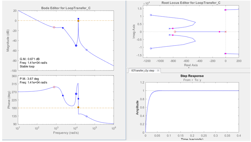
Figure 3‑24: Root locus for Controlled Current SEPIC.
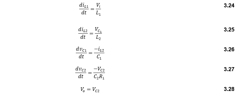
The PI coefficients are Kp = 0.00017814, and Ki = 0.1268, and the simulation results are shown below.