The number of statistical features used for this project was 33, which made the size of the matrix (76×33).

The features in the feature matrix included:

1. Mean
2. Median
3. Standard Deviation/Variance (S.D.)
4. Mean Absolute Deviation (MAD)
5. Quantiles or Percentiles
6. Interquartile Range (IQR)
7. Skewness
8. Kurtosis
9. Signal Entropy
10. Dominant Frequency Features
11. Bandpowers or Wavelet Features

The Feature Matrix was then used for creating test and train sets for data classification. Before doing that, the feature matrix needed a “Labeled Column,” which included the label for each patient represented by each row of the (76×33) Feature Matrix. Concatenating the labeled column to the Feature Matrix made the Feature Matrix size (76×34).

The labeled column consisted of the true class of the subject, which can be known from the original dataset. When the class of the patients is predicted, the predicted data will be compared to the labeled or true data to find the accuracy, precision, and other performances of the ML Algorithm used. Using the ‘KFold” technique from MATLAB, 5 Training and five respective testing folds were created from the dataset.

In each fold, 80% of the data was taken in the training set, while 20% of the data was chosen for the Testing Set. The training folds were used by the MATLAB Classification Learner Toolbox to create trained models based on various algorithms.

The following figure shows a screenshot of the MATLAB classification learner after training “Train_Fold 01”:

 

 

 

 

 

 

 

 

 

 

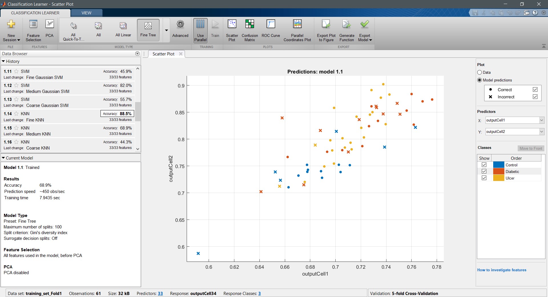
In MATLAB Classification Learner, the user can choose the type of algorithm they want to use to train their model.

In this case, all the available classifier algorithms were used to train the model, and the four best-performing algorithms were chosen. Fine k-Nearest Neighbor (FKNN), Quantum Support Vector Machine (SVM), Medium Gaussian Support Vector Machine (MGSVM), and Cubic Support Vector Machine (CSVM) were the chosen algorithms based on their high performance in the “Training Accuracy”.

Before finalizing the Training, the train sets were run several times. Even the folds were increased to 10 folds (which reduced the test_fold size due to the inherent characteristics of the “KFold” method) that are checked for performance. It was noticed that increasing the number of folds reduced the size of test_fold; the aim was to take it as 20% of the whole dataset.

It was further noticed that running the Classification Learner each time, the performance of the algorithms changes, but on average, the four chosen algorithms performed way better than others. So, 20 trained models were created from 5 training folds, four from each fold as trained under four different algorithms.

Each testing fold was tested against the trained models generated from its batch of training fold, e.g., testing fold one was tested against the four models created from the training fold 1. If a testing fold was tested against a training fold from a different batch, the performance was quite high (nearly 100%) but biased since all or most of the testing data are already present in that training fold, biasing the testing algorithm into unreasonably high performance.

The smart code developed by the team for appending labeled data to the Feature Matrix, Cross-Validation partition (CVpartition) and model testing printed out three crucial results after testing the “test_Fold” against a compatible training model,

• A two-column array representing a side by side presentation of the known and the predicted values
• The corresponding “Confusion Matrix.”
• “Accuracy,” “Precision,” “Recall” and “F1 Score”

The following figure illustrates the output of the testing of a test_fold against a train_model from the same batch:

 

 

 

 

 

 

 

 

 

 

 

 

 

 

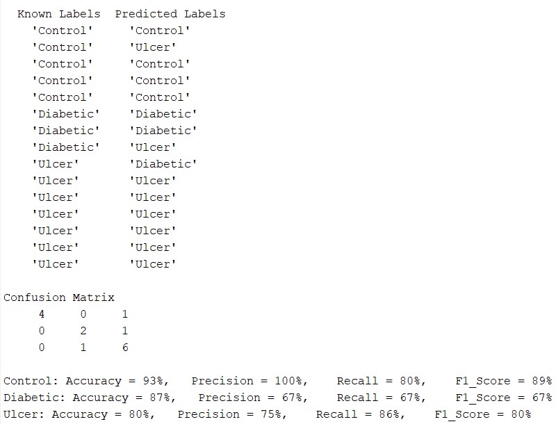
Here, from the figure above, it can be noticed that the Confusion Matrix has been created based on the relation between the known and the predicted labels. In this case, one “Control” subject was confused as “Ulcer,” one “Diabetic” subject was confused as having Ulcer, and one “Ulcer” subject was confused as a “Diabetic” subject. This has been represented in the Confusion Matrix in a well-arranged fashion.

MATLAB can generate its own, good looking Confusion Matrix through the command “Confusionchart(known_labels, predicted_labels).” This command once again affirms that the Confusion Matrix is constructed based on the Known and Predicted Labels. Testing the same test_fold (test_fold_01) against the “trainedmodel01_CSVM”, Matlab generates the same confusion matrix like the one generated by the code, shown in the figure below:

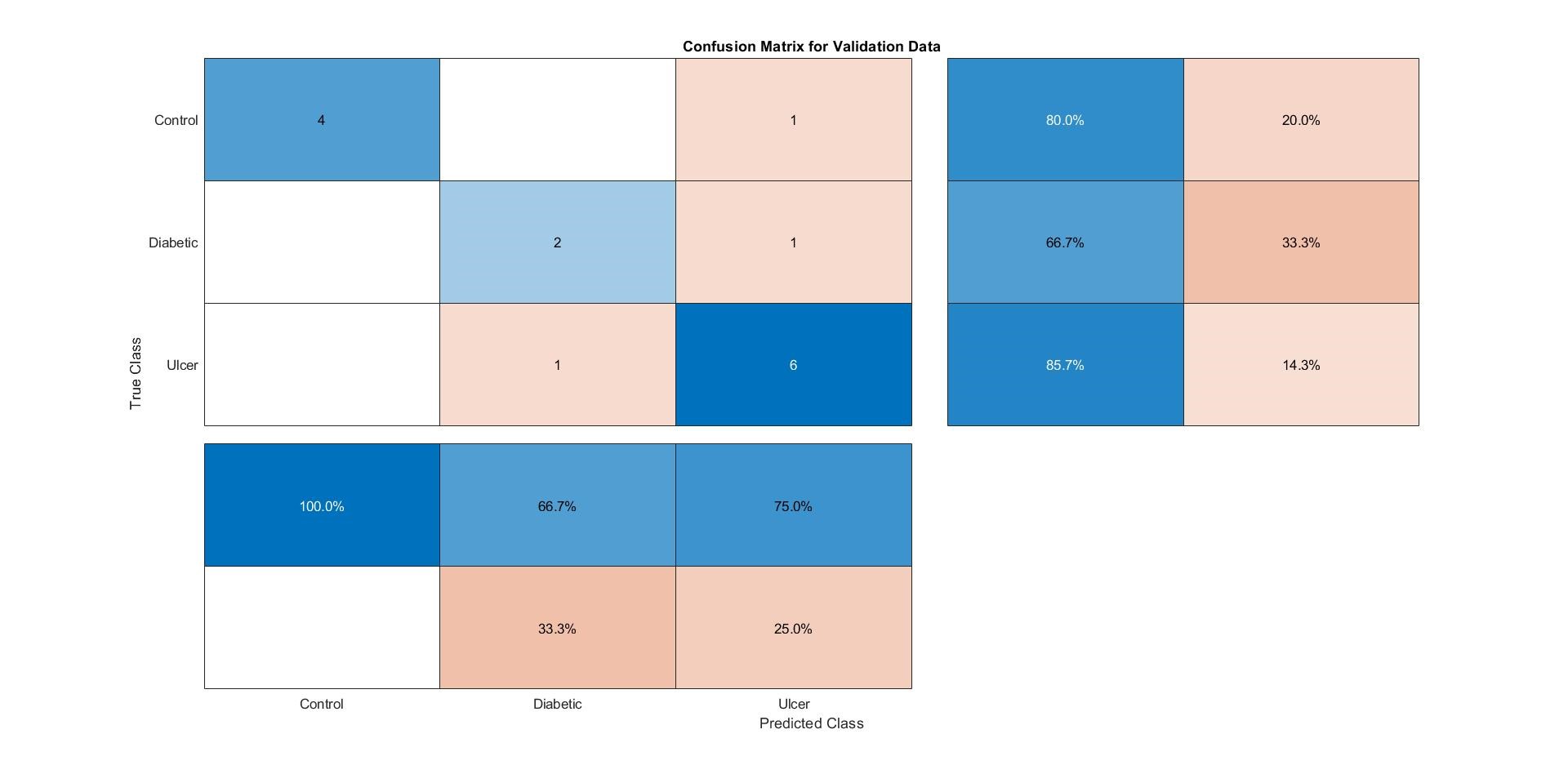
Note that the Matlab generated confusion matrix also provided with the “Precision” and the “Recall” parameters. Confusion Matrices and the other performance indicators were measured for all trained models, and the results were tabulated in an excel file to compare the performances among the four best-performing algorithms, as a whole and per class (Control, Diabetic, or Ulcer).

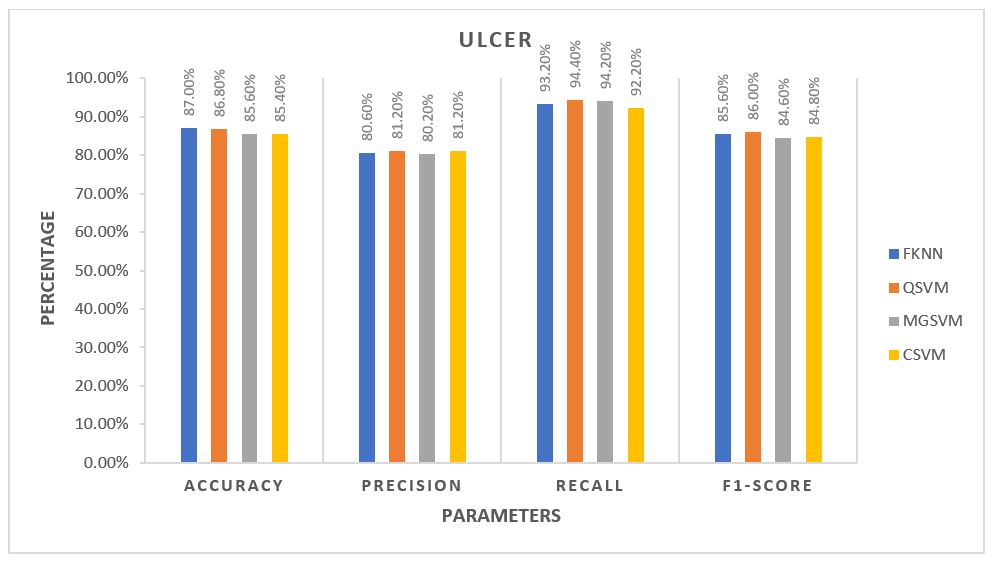
For each algorithm, the average of all five folds was calculated and plotted against each other. The plots are provided in the 3 figures below.

 

 

 

 

 

 

 

 

 

 

 

 

 

 

 

 

 

 

 

 

 

 

 

 

 

 

 

 

 

 

 

 

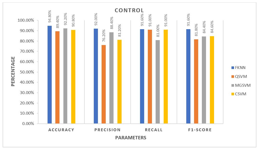
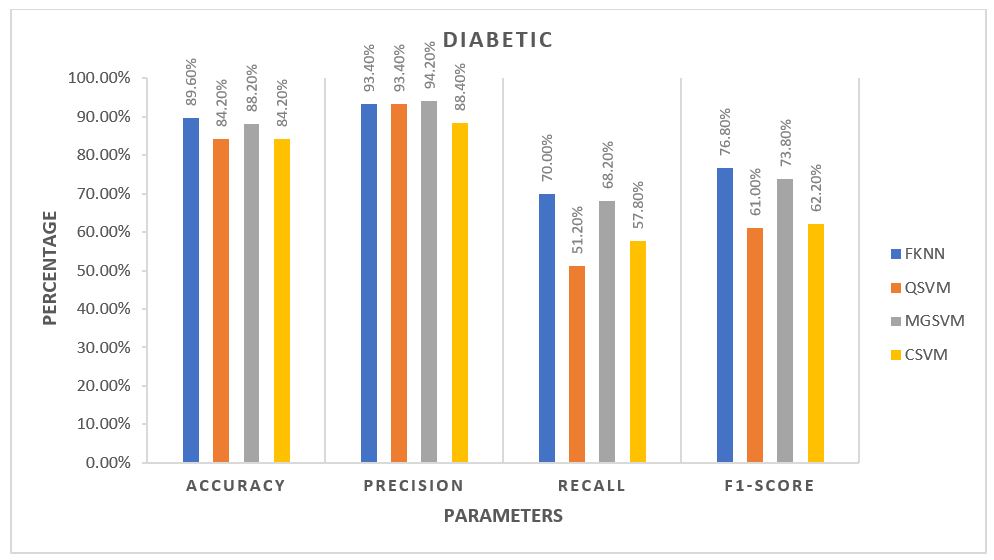
From the plots, for Control Subjects, the Fine k-Nearest Neighbour or FKNN algorithm performed better than the rest on average. For the other two classes of subjects, FKNN performed the best on average, making it most suitable for our project to test any unknown data, three other SVM based algorithms being the 2^nd choices.

Note that so far, the test data have been formed from the known data itself by forming 80-20 fold. Now, after we have roughly determined the best performing algorithms for this task, they can also be safely used to classify and predict unknown vGRF data outside this set.

The performance level also varied largely among the subject classes, which is conspicuous from table below, which shows the best performing algorithms based on patient class and parameters along with overall best Performances:

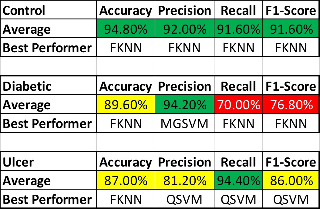
The average performance for the Control subjects was more than 90%, and FKNN was the winner in all cases. Ulcer patients showed an average performance of about 85% across various parameters. The performance was not as good as the Control Subjects but still much better than the Diabetic Patients. For the Ulcer patients, QSVM was the leading algorithm, while FKNN was trailing behind closely.

 

The main reason behind the lower accuracy among the Diabetic subjects is that being the middle class, many of their features are same as the Control subjects (since their Diabetic is not so severe, vGRF did not get altered too much) while many other features are same as the Ulcer patients (since Ulcer patients are also Diabetic patient but in critical condition). The main way to solve this problem is to,

• Gather more labeled data for training: This dataset contains only 76 data points, which is not nearly efficient for supplying the system with many distinct features. As a rule of thumb, 500+ subjects will be a sufficient number to boost ML Accuracy and Preciseness.
• Add More Statistical Features to the Feature Matrix: The current Feature Matrix has 33 statistical parameters as the features, which are acting as representatives for the dataset. Adding more statistical features will help the MATLAB classifier classify the subjects with more Accuracy and Precision.